| Home |
| News |
| Description |
| Papers |
| Source code |
| MEPX Software |
| Videos |
| Screenshots |
| User manual |
| Links |
| Contact |
| Download | User manual | Videos | What is new |
How to install Multi Expression Programming X
Windows 7, 8, 10, 11 (64-bit)
Just download the program from here:
mepx_win64.zip (2.45 MB)
unzip the archive and run the mepx.exe application. There is no installation kit. Please remember where you saved it so that you can run it next time.
Apple macOS / OSX (64-bit) (version 10.13 or newer; Intel and Apple Silicon)
Download the program from here:
mepx_macos.zip (4.4 MB)
It is .zip archive. Double-click it in Finder. It should be decompressed in the same folder as the zip archive. Open it from there (you should right click the icon and choose Open command).
Ubuntu (64-bit) (tested on Ubuntu 18)
Download the program from here:
mepx.deb (2.23 MB)
Install the program with Ubuntu Software Center.
If the icons are not shown on buttons, please open a Terminal and run the following command (this will display icons on buttons - which are disabled by default):
gsettings set org.gnome.settings-daemon.plugins.xsettings overrides "{'Gtk/ButtonImages': <1>, 'Gtk/MenuImages': <1>}"Test data
Test projects (taken from PROBEN1 and other datasets) can be downloaded from: MEPX test projects on Github. Just download a .xml file and press the Load project button from MEPX to load it.
User manual
- Quick start
- Data
- Parameters
- Results
- Use cases
- The format of the project files
- Running from the command line
- Integrating MEPX into other programs
- MEPX formulas as Excel functions
- Reporting problems
1. Quick start
- Select Data panel.
- Select Training data panel.
- Press the Load training data button and choose a csv or text file. Data must be separated by blank space, tab, comma or semicolon.
- Select Parameters panel. Modify some parameters if needed. For instance, one could modify code length, number of subpopulations, the (sub)population size, number of generations etc. Also, specify the problem type (regression or binary classification).
- Press the Start button from the main toolbar.
- Read the results from the Results panel.
- You can also save the entire project (data, parameters, results) by pressing the Save project from the main toolbar.
2. Data
The analysis is performed on tabular data. Data must be complete (no missing values).
There are 3 different types of data: Training, Validation, and Test. The training stage of the algorithm is performed on Training and (optionally on Validation data). At the end of the search process, the best solution (on Validation data - if present, if not on Training data) is tested against Test data.
The last value(s) (Target(s) column(s)) on each row is the target (expected output). Test data can be without an output (they may have fewer columns than training data).
The symbolic regression and time-series problems may have one output or more than one output. (More than one output is only allowed starting with version 2023.02.16)
Data for classification problems can have 1 output (1 column as output) only (but the generated programs for multi-class classification can have multiple outputs - see below).
For classification problems, the last column may contain only integer values (2 distinct values for binary classification or more for multi-class classification). Starting with version 2022.7.19, any integer values are accepted as output for classification problems. Previously, only continuous, integer values, starting with 0 were accepted as output for classification problems.
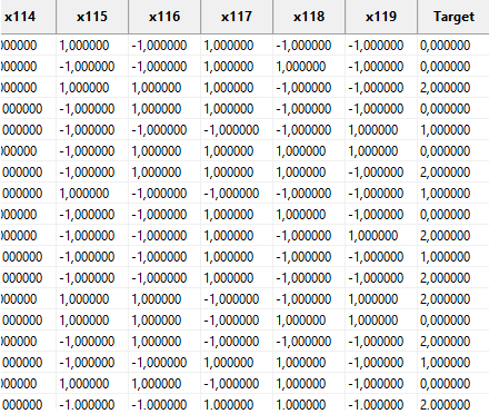
It is also possible that the output for classification problems to be loaded from files in one-of-m format. For instance, if the problem has 5 classes, the output consists in 5 binary values, one of them being set to 1 and all others being set to 0 (example: 0 1 0 0 0).
Training data is compulsory. The others (validation and test) are optional.
Alphanumeric values can be loaded into MEPX.
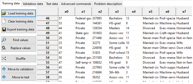
Alphanumeric values must be converted to numerical values before running the analysis. You have several specialized buttons for that:
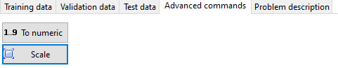
- To numeric - which will do an automatic conversion of alphanumerical values to integer values. The first alphanumerical value will be converted to 0, the second (distinct one) to one, and so on.
- Replace values - which will replace some values (alphanumeric with numeric). Find and replace works with regular expressions too.
- Export all data - which exports all data (Training + Validation + Test).
The user can also scale numerical values to a given interval.
2.1. Loading data
Data are loaded from csv, txt or other text files. The user can load data by pressing the Load button from the Training, Validation or Test page.
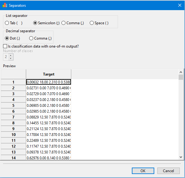
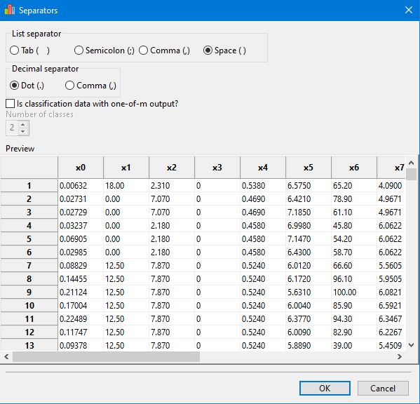
Import data window helps the user to specify which list separator, decimal separators and the number of classes (only for the one-of-m format of the output)
Values must be separated by blank space, tab, semicolon (;) or comma (,).
Values cannot be separated by multiple different separators (for example comma and space).
Consecutive separators are treated as one.
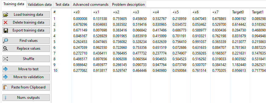
If the separators are correct, the data will appear in tabular format, as bellow:
For classification data with the output in one-of-m format, the user must specify the correct number of classes.
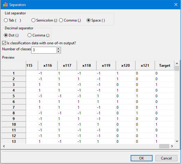
This setting has no effect in the Import data window, but, on the main page, the Target column is computed and displayed correctly:
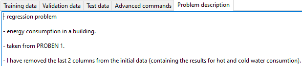
2.2. Problem description
A description of the problem can also be given and it will be saved as part of the project.
3. Parameters
3.1. Data type
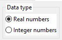
Can be:
- Real numbers - the underlying data type for inputs, programs, output is the double (64 bit real numbers).
- Integer numbers - the underlying data type for inputs, programs, output is the long long (64 bit integer numbers). Valid only for symbolic regression and time series problems. Only a limited set of mathematical functions can be used here.
3.2. Problem type
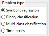
Can be:
- Symbolic Regression (sometimes called function fitting) with one or more outputs.
- Binary classification (with 2 classes)
- Multi-class classification (with 2 or more classes)
- Time series (univariate and multivariate)
Data for time-series can have 1 column or multiple columns. All columns are considered targets for time-series. (Multiple columns are permited only starting with version 2023.02.16.)
3.3. Error (Fitness) function
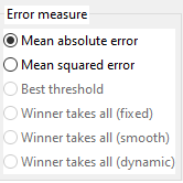
The algorithm will try to minimize the error.
Symbolic Regression
For symbolic regression problems, the fitness is:
- Mean Absolute Error (sum of absolute errors for each data (that is the difference between Target and the actual Output) divided by the number of examples)
- Mean Squared Error (sum of squared errors divided by the number of examples).
Classification
For classification, problems the fitness is computed in multiple ways depending on the problem or strategy. However what we report, in the resulting tables, is the percentage of incorrectly classified data (the number of incorrectly classified examples divided by the number of examples and multiplied by 100).
A classification problem with 2 classes can be solved by selecting either binary classification or multi-class classification.
Binary classification uses a threshold for making the distinction between classes. Values less or equal to the threshold are classified as belonging to class 0 and the others are classified as belonging to class 1.
In the case of binary classification, the threshold is computed automatically (because of that, binary classification can be slower sometimes).
For multi-class classification there are 4 strategies:
- Winner takes all - fixed positions -the outputs are assigned to groups of genes and the gene encoding the expression having the first maximal value will provide the class for that data.
- Winner takes all - fixed positions - smooth fitness
- Winner takes all - best genes
- Closest class
Time Series
For time series problems, the fitness is computed differently on training, validation and testing.
First of all, the training data is transformed to a matrix having (Window Size + 1)*Num Outputs columns and Num Training data - Window Size rows. This is done by considering each consecutive Window Size values as input and the next one as Target.
During evolution, the newly obtained matrix is used as training data. The error is computed as a regular Symbolic Regression.
At the end of each generation, the best function obtained on Training is applied on the Validation set. We actually want to validate the formula obtained on training.
Thus, again we construct a matrix, but in a different way. Instead of considering each consecutive values from Validation as input, we build the matrix dynamically considering the previously predicted values on Validation. Of course, the first row is made from the last Window Size values from Training (as input) and the first value from Validation (as Target). The error between predicted and the Target is computed as in the case of Symbolic Regression.
At the end of evolution, the best function from Validation is applied on the Test set, in the same manner as for the Validation set. The first row here is generated by taking the last Window Size values from Validation (or from Training if the Validation is empty).
3.4. Other parameters related to data
If use validation set is checked then, at each generation, the best individual on Training is run against the Validation data, and the best such individual (from those tested against the validation set) is the output of the program (and will be applied on the Test data).
Note that, when the Validation data is used, the output of the MEPX is the best solution on Validation, not the best on Training. During evolution, one may see improvements on Training error, but the final solution might not perform so well on Training because the best for Validation is the final solution. Still, the Validation data is useful to prevent overfitting on Training.
It is possible to run the optimization on a smaller set of Training data. In such case, you have to set the Random subset size percent to a value smaller than 100%. The training set is changed after Num generations for which random subset is kept fixed.
3.5. Time series parameters
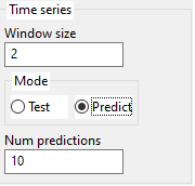
The formula is trained on the Training set and then it is used to predict values on the Validation set. It is highly recommended to have Validation set, otherwise, the results can be poor due to overfitting on Training.
MEPX will internally transform columns of training data into a matrix having (Window size + 1)*Num outputs columns. (the last Num outputs columns are the Targets).
After discovering the formula, it can be used either to predict values on the Test set or to predict future values, depending on the Time series mode setting.
The user can also specify how many future values to predict.
3.6. Functions (or mathematical operators)
Here is the list of operators that can appear in the result.
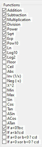
These are classic arithmetic operators +, -, *, ... nothing new here.
Only some mathematical functions are available if the data type is integer numbers.
Modulus can be used for both real and integer data types.
Note that trigonometric operators work with radians.
Do not confuse them with genetic operators used by the MEP algorithm.
3.7. Constants
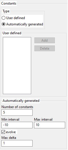
To enable constants, one must define a probability greater than 0 for constants. You cannot edit that probability directly, but constants_probability + operators_probability + variables_probability = 1. So if you define a value for probability for operators or variables such that their sum is less than 0, you will get a greater than 0 value for constants.
Constants can be user-defined or generated by the program (over a given interval). Generated constants can be kept fixed for all the evolution or they can also evolve. Mutation of constants is done by adding a random value between [-max delta, +max_delta].
3.8. The algorithm
The data analysis cannot be made instantaneously due to the complexity of the problem. This is why a special algorithm inspired by biology is used. The algorithm works with multiple potential solutions that are modified (hopefully improved) along with a number of generations.
MEPX uses a steady state model with multiple subpopulations. Steady-state means that inside one subpopulation, the worst individuals are replaced with newer ones (if the newer are better).
At the end of each generation, the best individual in that generation is tested against the Validation set. The best on Validation is retained and tested, at the end of the search process against Test set.
Parameters for the algorithm are specified in the below image:
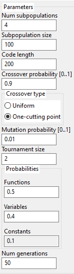
The user may specify the number of subpopulations. Each subpopulation will run independently from the others and, after one generation, they will exchange few individuals.
Genetic operators (crossover and mutation) are classic ... nothing new here.
It is possible to specify how often the variables, operators, and constants should appear in a chromosome. This is done probabilistically. If you want more operators to appear, please increase the operators' probability. More operators mean more complex expressions.
The sum of functions (operators) probability, variables probability and constants probability must be 1. The constants' probability is computed automatically as 1 - the sum of the other 2 probabilities.
3.9. Runs
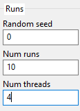
Random seed - It is also possible to specify the initial seed of the first run (consecutive runs will start from the previous seed + 1).
Num runs - Usually multiple runs must be performed for computing some statistics.
Num threads - Specify the number of processor cores used for running the algorithm. Each subpopulation is run on a thread. This can increase the speed of analysis significantly. If you have a quad-core processor with hyper-threading, you may set the number of threads to 8. For best results make sure that the number of subpopulations is a multiple of the number of threads.
4. Results
The following results are displayed:
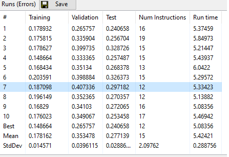
4.1. Error
Error for the entire training, validation, and test set.
In the case of classification problems, the number of incorrectly classified data (in percent) is shown.
The number of effective instructions of the best program (in the simplified form) and the running time required to obtained the solution are also displayed in this table.
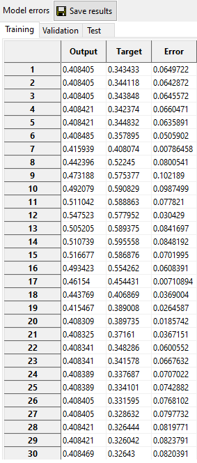
4.2. Model
Obtained value for each data in the training, validation, and test set (also called Model or Output).
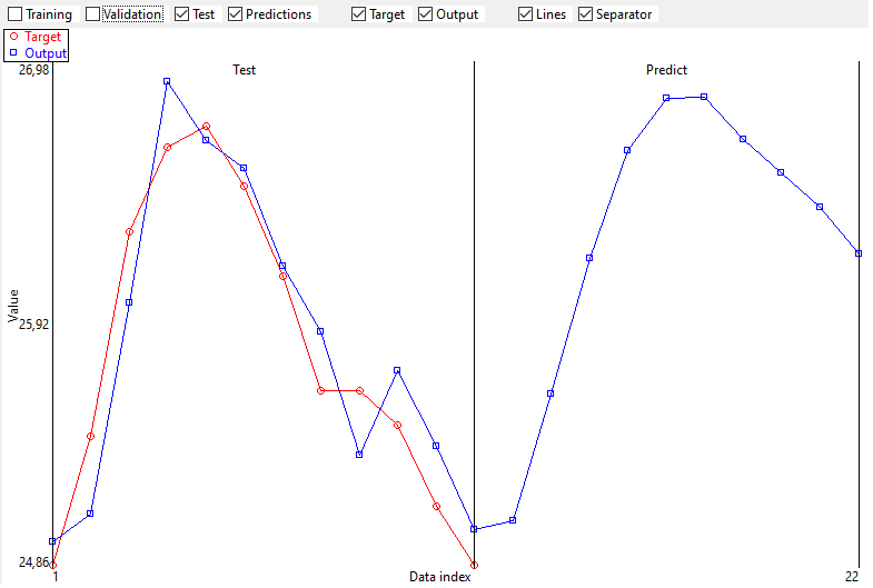
4.3. Output and Target graphically
The target and the output are represented graphically too.
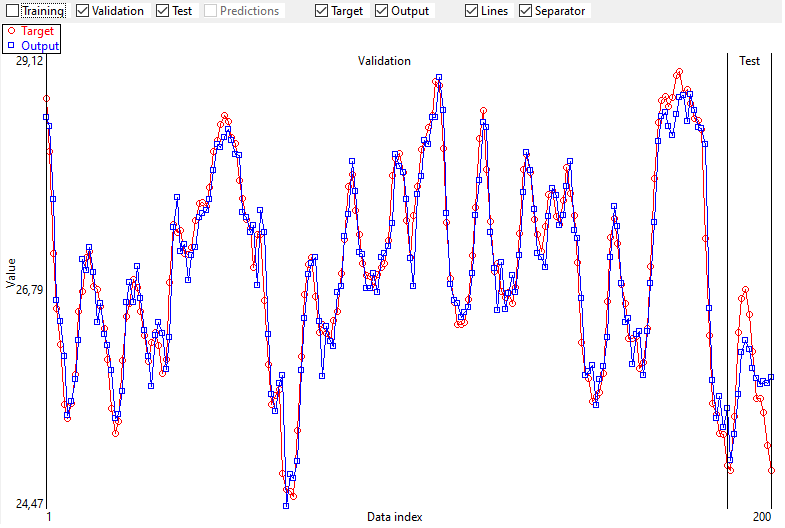
Predictions of future values are also represented graphically if the setting of Time Series mode is Predict.
4.4. Source code
C/C++, Excel VBA, Python or Latex source code of the best solution. This code can be simplified to show only instructions that generate the output (remember that not all genes of a chromosome participate to the solution - these genes are called introns). Note that there is no simplification in the case of multi-class classification.
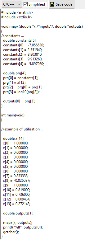
Excel VBA code can be used to create a custom formula in Excel.
One can analyze new data directly from Excel with the formula discovered by MEPX.
A movie with this feature is here on YouTube.
Another movie with univariate time-series predictions in Excel is here on YouTube.
Another movie with multivariate time-series formulas loaded in Excel is here on YouTube.
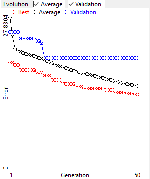
4.4. Evolution
Evolution of the fitness for the best individual in the population, the average fitness of the population and the fitness on the validation set (only from version 2022.11.4.2).
Note that, for classification problems, the fitness is not always computed as the number of incorrectly classified data.
5. Use cases
Particular settings for each type of problem are described in this section.
5.1. Symbolic regression
Data must be in tabular format. Last columns are the target. Target is compulsory for Training and Validation, but not for Test set.
Problem type must be set to Symbolic Regression.
5.2. Classification
Data must be in tabular format. Last column is the target class. Target is compulsory for Training and Validation, but not for Test set.
Classes must be represented as integer numbers. Starting with version 2022.7.19, any integer numbers are accepted as target. Previously, the target should have been integer values between 0 and Number of classes - 1.
Data can be loaded from files where the target is represented in 1-of-m format (0 0 1 0), but will be transformed into 1 column during import.
Problem type must be set to Binary classification or Multi-class classification.
5.3. Time series
Problem type must be set to Time series.
Window size must be set. This parameter could influence the quality of prediction.
Predict mode must be set. First try to predict on Test then change to predict new data.
If Predict mode is Predict new data then, the Number of predictions must be set.
6. The format of the project files
Projects can be saved/loaded to/from .xml files which is the default format of the MEPX.
The xml file has a tree structure. The root node is named project.
Inside project we have other nodes like mepx_version, problem_description, algorithm.
Inside the algorithm node we have training, validation, test, parameters, operators, results, etc
Main structure of the .xml files is the following:
<?xml version="1.0"?>
<project>
<mepx_version> </mepx_version>
<problem_description> </problem_description>
<algorithm>
<training> </training>
<validation> </validation>
<test> </test>
<variables_utilization> </variables_utilization>
<parameters> </parameters>
<constants> </constants>
<operators> </operators>
<results> </results>
</algorithm>
</project>
7. Running from the command line
MEPX can be run in dual mode:
- If you run it with no parameters the program will create the standard user interface.
- If you supply with 2 or 3 parameters (see below), the program will create no interface and it will just read the data from a file and it will output the results in another file.
The command line has this form:
mepx.exe input.xml output.xml
, where input.xml is a valid MEPX project.
If the files are not in the same directory, please make sure that you give the full path for them!
If you want to stop it earlier, run this command:
mepx.exe input.xml output.xml stop_file_name
Note: Last parameter is optional and is used only if you want to stop the search process earlier.
8. Embedding the MEPX in your application
If you want to embed the program in your Windows application you can create a new process using the CreateProcess function from Windows API.
When the process is over you should read the results from the output.xml file. You can check if the process is almost over by checking for the existence of output.xml. The existence of the file does not guarantee that the writing of data is over. You can check of the file writing is over by looking for the </project> tag in the xml file. Or you can simply check if the file can be renamed.
The search process can take a few milliseconds or minutes or hours depending on the data to be analyzed. If you want to stop the search process before it naturally ends, you should create a file (stop_file_name)) which you specified as the last parameter of the command line. The program will check for the existence of that file and will stop the search when that file is found. Make sure that you delete this file if you previously created it with another search!
9. Use MEPX formulas as Excel functions
- First, run MEPX on some data to obtain the formula.
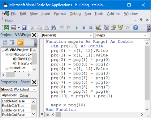
- Go to the Results tab and show source code in Excel VBA (Visual Basic for Applications).
- Start Excel and load some data. They must have the same number of columns as the data used by MEPX to discover the formula. The target column may or may not exist.
- Now we will create a custom Excel formula with the code generated by MEPX.
- Press Alt+F11 to open the Excel VBA editor for Windows. On Mac, you should press Fn+Alt+F11.
- Copy/Paste the formula generated by MEPX into the VBA editor.
- Save the Excel file as xlsm (Excel Macro-Enabled Workbook). This format is required because now we have some code in our xlsx file. Is not only data. It is VBA code too.
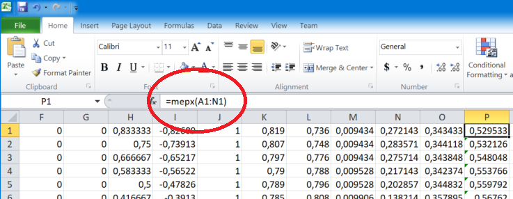
- Now we have a new Excel formula named mepx that we will use for our data. The formula accepts a Range of cells as the parameter (e.g. A1:D1). The formula can be applied for 1 row at a time.
- Go to Excel data file (press Alt+F11 to switch from data to code and vice-versa).
- Use the formula to compute the output.
A movie with this feature is here on YouTube.
Version 2021.10.29 or newer is needed to export formulas in VBA for Excel.
10. Reporting problems, bugs, comments
If you have problems with this program please save the project (by pressing the Save Project button from the main toolbar) and send it to mihai.oltean@gmail.com